Deep Learning vs. Machine Learning – how to tell the difference?

In recent years, Machine Learning, Deep Learning, and Artificial Intelligence have become buzz words. As a result, you can find them all over in marketing materials and advertisements of more and more companies.

But what are Machine Learning and Deep Learning? Also, what are the differences between them? In this article, I will try to answer these questions, and show you some cases of Deep and Machine Learning applications.

What is Machine Learning?

Machine Learning is a part of Computer Science that deals with representing real-world events or objects with mathematical models, based on data. These models are built with special algorithms that adapt the general structure of the model so that it fits the training data. Depending on the type of problem being solved, we define supervised and unsupervised Machine Learning and Machine Learning algorithms.

Supervised vs. unsupervised Machine Learning

Supervised Machine Learning focuses on creating models that would be able to transfer knowledge we already have about the data at hand to new data. The new data is unseen by the model-building (training) algorithm during the training phase. We provide an algorithm with the features’ data along with the corresponding values the algorithm should learn to infer from them (so-called target variable).

In unsupervised Machine Learning, we only provide the algorithm with features. That allows it to figure out their structure and/or dependencies on its own. There is no clear target variable specified. The notion of unsupervised learning can be hard to grasp at first, but taking a look at the examples provided on the four charts below should make this idea clear.

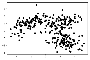
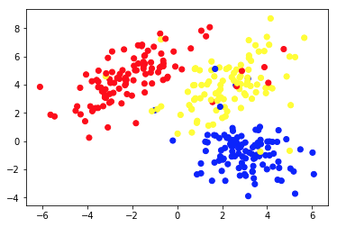
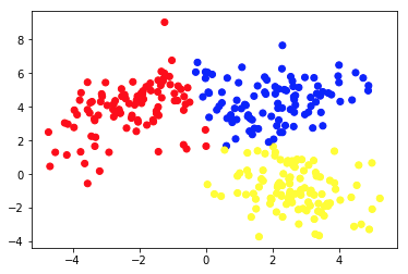
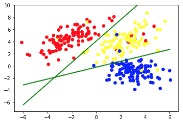
Chart 1a presents some data described with 2 features on axes x and y. The one marked as 1b shows the same data colored. We used the K-means clustering algorithm to group these points into 3 clusters, and colored them accordingly. This is an example of unsupervised Machine Learning algorithm. The algorithm was only given the features, and the labels (cluster numbers) were to be figured out.

The second picture shows Chart 2a, which presents a different set of labeled (and colored accordingly) data. We know the groups each of the data points belong to a priori. We use an SVM algorithm to find 2 straight lines that would show us how to split data points to fit these groups best. This split is not perfect, but this is the best that can be done with straight lines. If we want to assign a group to a new, unlabeled data point, we just need to check where it lies on the plane. This is an example of a supervised Machine Learning application.

Applications of Machine Learning models

Standard Machine Learning algorithms are created for handling data in a tabular form. This means that in order to use them we need some kind of a table. In such table rows can be thought of as instances of the object modeled (e.g., a loan). At the same time, the columns should be seen as features (characteristics) of this particular instance (e.g., monthly payment of the loan, monthly income of the borrower).

Table 1. is a very short example of such data. Of course, it does not mean that the pure data itself have to be tabular and structured. But if we want to apply a standard Machine Learning algorithm on some dataset, we usually have to clean, mix and transform it into a table. In supervised learning, there is also one special column that contains the target value (e.g., information if the loan has defaulted).

The training algorithm tries to fit the model’s general structure into these data. Said algorithm does that by tweaking the model’s parameters. That results in a model that describes the relationship between the given data and the target variable as accurately as possible.

It is important that the model not only fits the given training data well but is also able to generalize. Generalisation means that we can use the model to infer the target for instances not used during training. It is also a crucial feature of a useful model. Building a well-generalizing model is not an easy task. It often requires sophisticated validation techniques and thorough model testing.

loan_id	borrower_age	income_monthly	loan_amount	monthly_payment	default
1	34	10,000	100,000	1,200	0
2	43	5,700	25,000	800	0
3	25	2,500	24,000	400	0
4	67	4,600	40,000	2,000	1
5	38	35,000	2,500,000	10,000	0

Table 1. Loan data in a tabular form

People use Machine Learning algorithms in a variety of applications. Table 2. presents some business use cases allowing non-deep Machine Learning algorithms and models appliance. There are also short descriptions of the potential data, target variables, and selected applicable algorithms.

Use case	Data examples	Target (modeled) value	Algorithm/model  used
Recommendations of articles on a blog site	IDs of articles read by users, time spent on each of them	Preferences of users towards articles	Collaborative Filtering with Alternating Least Squares
Credit scoring of mortgages	Transactional and crediting history, income data of a potential borrower	Binary value showing if a loan will be repaid in full or it will default	LightGBM
Predicting churn of premium users of a mobile game	Time spent on playing daily, time since first launch, progress in the game	Binary value showing if a user is going to cancel subscription next month	XGBoost
Credit card fraud detection	Historical credit card transactions data – amount, place, date and time	Binary value showing if a credit card transaction is fraudulent	Random forest
Segmentation of customers of an internet store	Purchase history of loyalty program members	Segment number assigned to every customer	K-means
Predictive maintenance of a machine park	Data from performance, temperature, humidity, etc. sensors	One of the following classes – ‘fine’, ‘to observe’, ‘requires maintenance’	Decision tree

Table 2. Examples of Machine Learning use cases

Deep Learning and Deep Neural Networks

Deep Learning is part of Machine Learning in which we use models of a specific type, called deep artificial neural networks (ANNs). Since their introduction, artificial neural networks have gone through an extensive evolution process. That led to a number of subtypes, some of which are very complicated. But in order to introduce them, it is best to explain one of their basic forms – a multilayer perceptron (MPL).

Multilayer perceptron

Simply put, a MLP has a form of a graph (network) of vertices (also called neurons) and edges (represented by numbers called weights). The neurons are arranged in layers, and the neurons in consecutive layers are connected with each other. Data flows through the network from the input to the output layer. The data is then transformed at the neurons and the edges between them. Once a data point passes through the whole network, the output layer contains the predicted values in its neurons.

Every time a chunk of the training data passes through the network, we compare the predictions with the corresponding true values. That lets us adapt the parameters (weights) of the model to make predictions better. We can do it with an algorithm called backpropagation. After some number of iterations, if the structure of the model is well designed specifically to tackle the Machine Learning problem at hand.

Obtaining a high-accuracy model

Once enough data has passed through the network multiple times, we obtain a high-accuracy model. In practice, there are plenty of transformations that can be applied at neurons. That makes the ANNs very flexible and powerful. The power of ANNs comes at a price, though. Usually, the more complicated the structure of the model, the more data and time it requires to train it to high accuracy.

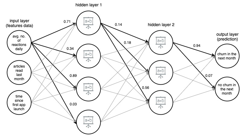
Image 1. (draw.io) Structure of a 4-layer artificial neural network, predicting if a user of a news app will churn next month, based on three simple features.

For clarity, weights have been marked only for selected (bolded) edges, but every edge has its own weight. Data flows from the input layer to the output layer, passing through 2 hidden layers in the middle. On each edge, an input value is multiplied by the edge’s weight, and the resulting product goes to the node the edge ends at. Then, in each of the nodes in the hidden layers, the incoming signals from edges are summed up and then transformed with some function. The result of these transformations is then treated as an input to the next layer.

In the output layer, the incoming data is again summed up and transformed, yielding the result in the form of two numbers – the probability that a user will churn from the app in the next month, and the probability that they will not.

Advanced types of neural networks

In neural networks of more advanced types, the layers have a much more complex structure. They consist of not only simple dense layers with one-operation neurons known from MLPs, but also much more complicated, multi-operation layers like convolutional, and recurrent layers.

Convolutional and recurrent layers

Convolutional layers are mostly used in computer vision applications. They consist of small arrays of numbers that slide over the pixel representation of the image. Pixel values are multiplied by these numbers and then aggregated, yielding new, condensed, representation of the image.

Recurrent layers are used to model ordered sequential data like time series or text. They apply much complicated multi-argument transformations to incoming data, trying to figure out the dependencies between the sequence items. Nevertheless, no matter the type and structure of the network, there are always some (one or more) input and output layers, and strictly defined paths and directions in which the data flows through the network.

In general, Deep Neural Networks are ANNs with multiple layers. Images 1, 2, and 3 below show architectures of selected deep artificial neural networks. They were all developed and trained at Google, and made available to the public. They give an idea on how complex high-accuracy deep artificial networks used today are.

These networks have enormous sizes. For example, partially shown in Image 3 InceptionResNetV2 has 572 layers, and more than 55 million parameters in total! They have all been developed as image classification models (they assign a label, e.g. ‘car’ to a given image), and have been trained on images from the ImageNet set, consisting of more than 14 million labeled images.

Image 2. Structure of NASNetMobile (keras package)

Image 3. Structure of XCeption (keras package)

Image 4. Structure of a part (around 25%) of InceptionResNetV2 (keras package)

In recent years we have observed great development in Deep Learning and its applications. Many of the ‘smart’ features of our smartphones and applications are the fruit of this progress. Although the idea of ANNs is not new, this recent boom is a result of meeting a few conditions. First of all, we have discovered the potential of GPU computing. Graphical processing units’ architecture is great for parallel computation, very helpful in efficient Deep Learning.

Moreover, the rise of cloud managed services has made access to high-efficiency hardware much easier, cheaper, and possible on a much bigger scale. Finally, the computational power of the newest mobile devices is large enough to apply Deep Learning models, creating a huge market of potential users of DNN-driven features.

Applications of Deep Learning models

Deep Learning models are usually applied to problems that deal with data that do not have a simple row-column structure, like image classification or language translation, as they are great at operating on unstructured and complex-structure data these tasks handle – images, text, and sound. There are problems with handling data of these types and sizes with classical Machine Learning algorithms, and creating and applying some deep neural networks to these problems have caused tremendous developments in the fields of image recognition, speech recognition, text classification, and language translation in the last few years.

Application of Deep Learning to these problems was possible due to the fact that DNNs accept multi-dimensional tables of numbers, called tensors, as both input and output, and can track the spatial and temporal relationships between their elements. For example, we can present an image as a 3-dimensional tensor, where dimension one and two represent the resolution of the digital image (so have the sizes of the image width and height, respectively), and the third dimension represents the RGB color coding of each of the pixels (so the third dimension is of size 3).

This allows us to not only represent all the information about the image in a tensor but also keep the spatial relationships between pixels, which turns out to be crucial in the application of so-called convolutional layers, crucial in successful image classification and recognition networks.

Neural network flexibility in the input and output structures helps also in other tasks, like language translation. When dealing with text data, we feed the deep neural networks with number representations of the words, ordered according to their appearance in the text. Each word is represented by a vector of one hundred or a few hundred numbers, computed (usually using a different neural network) so that the relationships between vectors corresponding to different words mimic the relationships of the words themselves. These vector language representations, called embeddings, once trained, can be reused in many architectures, and are a central building block of neural network language models.

Examples of Deep Learning models use

Table 3. contains examples of applying Deep Learning models to real-life problems. As you can see, problems tackled and solved by Deep Learning algorithms are much more complex than tasks solved by standard Machine Learning techniques, like those presented in Table 1.

Nevertheless, it is important to remember that many of the use cases Machine Learning can help with businesses today do not require such sophisticated methods, and can be solved more efficiently (and with higher accuracy) by standard models. Table 3. also gives an idea on how many different types of artificial neural networks layers there are, and how many different useful architectures can be constructed with them.

Use case	Data	Target/result of the model	Algorithm/model used
Image classification	Images	Label assigned to an image	Convolutional Neural Network (CNN)
Image detection by self-driving cars	Images	Labels and bounding boxes around objects identified on images	Fast R-CNN
Sentiment analysis of comments in an online store	Text of online comments	Sentiment label (e.g., positive, neutral, negative) assigned to each comment	Bidirectional Long-Short Term Memory (LSTM) Network
Harmonization of a melody	MIDI file with a melody	MIDI file with this melody harmonized	Generative Adversarial Network
Next word prediction in an online email editor	Very large chunkof text (e.g., dump of all Wikipedia articles in English)	A word that fits as the next one the text written so far	Recurrent Neural Network (RNN) with an Embedding layer
Text translation into another language	Text in Polish	The same text translated to English	Encoder – Decoder Network built with recurrent neural network (RNN) layers
Transfer of Monet’s style to any image	Set of images of Monet’s paintings, and a set of other images	Images modified to look as painted by Monet	Generative Adversarial Network

Table 3. Examples of Deep Learning use cases

Advantages of Deep Learning models

Generative Adversarial Networks

One of the most impressive applications of Deep Neural Networks came with the rise of Generative Adversarial Networks (GANs). They were introduced in 2014 by Ian Goodfellow, and his idea has since been incorporated in many tools, some with astonishing results.

GANs are responsible for the existence of applications that make us look older in photos, transform images so that they look as if they were painted by van Gogh, or even harmonize melodies for multiple instrument bands. During training of a GAN, two neural networks compete. A generator network generates an output from random input, while the discriminator tries to tell generated instances from real ones. During training, the generator learns how to successfully ‘fool’ the discriminator, and eventually is able to create output that looks as if it was real.

Powerful deep neural networks in mobile apps

It is important to note that even though training a deep neural network is a very computationally expensive task and can take a long time, applying a trained network to do a specific task does not have to be, especially if it is applied to one or a few cases at once. Actually, today we are able to run powerful deep neural networks in mobile applications on our smartphones.

There are even some network architectures specifically designed to be efficient when applied on mobile devices (e.g., NASNetMobile presented in Image 1). Even though they are much smaller in size compared to the state-of-the-art networks, they are still able to obtain a high accuracy prediction performance.

Transfer learning

Another very powerful feature of artificial neural networks, enabling wide use of the Deep Learning models, is transfer learning. Once we have a model trained on some data (either created by ourselves, or downloaded from a public repository), we can build upon all or part of it to get a model that solves our particular use case. For example, we could use a pre-trained NASNetLarge model, trained on the huge ImageNet dataset, that assigns a label to an image, make some small modifications on the top of its structure, train it further with new set of labeled images, and use it to label some specific type of objects (e.g. species of a tree based on the image of its leaf).

Perks of transfer learning

Transfer learning is very useful, as usually training a deep neural network that will perform some practical, useful tasks requires vast amounts of data and huge computational power. This can often mean millions of labeled data instances, and hundreds of graphics processing units (GPUs) running for weeks.

Not everyone can afford or has access to such assets, which can make it very hard to build a high-accuracy custom solution from scratch for, let’s say, image classification. Fortunately, some pre-trained models (especially networks for image classification and pre-trained embedding matrices for language models) have been open-sourced and are available for free in an easily-applicable form (e.g. as a Model instance in Keras, a neural networks API).

How to choose and build the right Machine Learning model for your application

When you want to apply Machine Learning to solve a business problem, you probably don’t need to decide on the type of the model right away. There are usually a few approaches that could be tested. It is often tempting to start with the most complicated models at first, but it is worth starting simple, and gradually increasing the complexity of the models applied. Simpler models are usually cheaper in terms of set up, computation time, and resources. Moreover, their results are a great benchmark to evaluate more advanced approaches.

Having such benchmarks can help data scientists to assess if the direction they develop their models in is the right one. Another advantage is the possibility of reusing some of the previously built models, and merging them with newer ones, creating a so-called ensemble model. Mixing models of different types often yields higher performance metrics than each of the combined models alone would have. Also, check if there are some pre-trained models that could be used and adapted to your business case via transfer learning.

More practical tips

First and foremost, whatever model you use, make sure that the data is handled properly. Keep in mind the ‘garbage in, garbage out’ rule. If the training data provided to the model is of low quality or has not been properly labeled and cleaned, it is very likely that the resulting model will also perform poorly. Also ensure that the model – whatever its complexity – has been extensively validated during the modeling phase, and in the end tested if it generalizes well to unseen data.

On a more practical note, make sure that the created solution can be implemented in production on the available infrastructure. And if your business can collect more data that could be used to improve your model in the future, a retraining pipeline should be prepared to ensure its easy update. Such a pipeline can even be set up to automatically retrain the model with a predefined time frequency.

Final thoughts

Don’t forget to track the model’s performance and usability after its deployment to production, because business environment is very dynamic. Some relationships within your data may change over time, and new phenomena can arise. They can, therefore, change the efficiency of your model, and should be treated properly. Additionally, new, powerful types of models can be invented. On one hand, they can make your solution relatively weak, but on the other, give you the opportunity to further improve your business and take advantage of the newest technology.

What is more, Machine and Deep Learning models can help you build powerful tools for your business and applications and give your customers an exceptional experience. Although creating these ‘smart’ features requires substantial effort, but the potential benefits are worth it. Just make sure you and your Data Science team try appropriate models and follow good practices, and you will be on the right track to empower your business and applications with cutting-edge Machine Learning solutions.

However, if you would like to create unique solutions with a machine learning development company, contact us! Together we will create a product that perfectly meets your requirements.

Sources:

• https://en.wikipedia.org/wiki/Unsupervised_learning
• https://keras.io/
• https://developer.nvidia.com/deep-learning
• https://keras.io/applications/
• https://arxiv.org/abs/1707.07012
• http://yifanhu.net/PUB/cf.pdf
• https://towardsdatascience.com/detecting-financial-fraud-using-machine-learning-three-ways-of-winning-the-war-against-imbalanced-a03f8815cce9
• https://scikit-learn.org/stable/modules/tree.html
• https://aws.amazon.com/deepcomposer/
• https://blog.keras.io/a-ten-minute-introduction-to-sequence-to-sequence-learning-in-keras.html
• https://keras.io/examples/nlp/bidirectional_lstm_imdb/
• https://towardsdatascience.com/how-do-self-driving-cars-see-13054aee2503
• https://towardsdatascience.com/r-cnn-fast-r-cnn-faster-r-cnn-yolo-object-detection-algorithms-36d53571365e
• https://towardsdatascience.com/building-a-next-word-predictor-in-tensorflow-e7e681d4f03f
• https://keras.io/applications/
• https://arxiv.org/pdf/1707.07012.pdf